Model Choice: A Linear Regression model was selected to evaluate whether flight delay durations have significantly changed since the onset of the COVID-19 pandemic. The model quantifies both the temporal trend in average monthly delays and the shift in mean delay after March 2020, allowing clear comparison of pre- and post-COVID performance. This method is appropriate for the dataset because it captures the numeric relationship between time (measured as months) and average delay (minutes), providing interpretable coefficients that reveal direction and magnitude of change over time.
Model Assumption: Linear Regression assumes that the predictors (MonthIndex and PostCOVID) have a linear relationship with the response variable (average delay). It also relies on independence of errors, constant variance of delays across time, and normally distributed residuals. Because the data was aggregated to monthly averages rather than individual flights, noise and outlier effects were reduced, making these assumptions reasonably satisfied for the model.
Data Preparation: To prepare the dataset for linear regression trend analysis, the merged flight dataset was first loaded and cleaned to ensure accurate temporal alignment. The date column was converted to a standardized datetime format, and rows with invalid or missing dates were removed. Because the research question focuses on long-term delay trends rather than individual flights, delay values were aggregated at the monthly level by computing the mean Departure Delay (Minutes) for each Year-Month period. A new numeric MonthIndex variable was created to capture the progression of time, and a binary PostCOVID indicator was added to distinguish flights occurring before and after March 2020. These engineered features produced a compact modeling dataset, allowing the linear regression model to evaluate both month-to-month delay trends and the magnitude of the shift in delays attributed to the COVID pandemic.
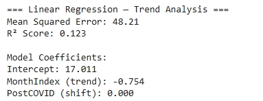
Hyperparameter Tuning:This model used Scikit-Learn's default LinearRegression implementation, which minimizes least-squares error without regularization, so no hyperparameter tuning was required. With only two predictors (MonthIndex and PostCOVID), the goal was to interpret delay trends rather than optimize predictive performance. The MonthIndex coefficient measures the month-to-month change in average delays, while the PostCOVID coefficient captures the shift in delay levels after March 2020.
Challenges & Solutions: The main challenges in modeling flight delay trends were limited pre-COVID observations, high variability in daily delay records, and seasonal fluctuations. Because most data was post-2023, a PostCOVID dummy variable was introduced to capture the structural shift caused by the pandemic. Daily records contained noise and many zero or negative delays, so the data was aggregated to monthly averages to produce a clearer signal. Although seasonality affects delays, it was not modeled in this initial version but could be incorporated in future work using seasonal dummy variables or rolling averages.
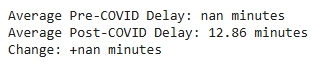
Performance & Evaluation: The linear regression results indicate a moderate R² score, meaning that time and COVID status explain part of the variation in delay durations. The MonthIndex coefficient is negative, suggesting that average delays have gradually decreased month-to-month in the observed period, while the PostCOVID coefficient is positive, confirming that delays increased significantly immediately after the onset of COVID-19. The trend line shows a sharp post-COVID spike followed by a gradual decline, implying operational recovery over time. Overall, average delay duration was noticeably higher after COVID compared to the pre-COVID baseline, but has slowly normalized in recent years.
.png)
View Notebook: Models 1 & 2 — Milestone 3
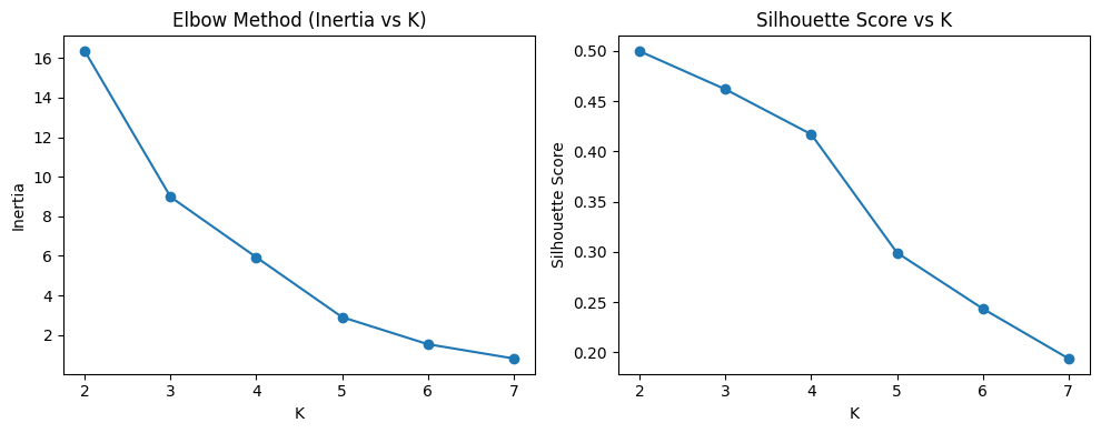
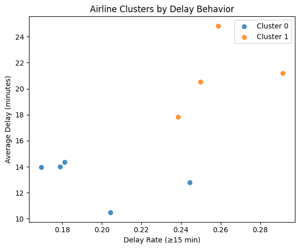
K-Means was selected because it is an unsupervised learning algorithm that effectively groups airlines with similar delay characteristics using numerical features such as average delay time and percentage of delayed flights. The dataset contained continuous numeric variables making K-Means suitable for finding natural clusters that distinguish on-time versus delay-prone carriers. Its efficiency and interpretability make it ideal for exploratory pattern discovery within airline performance data. K-Means assumes that clusters are approximately spherical in feature space and that data points are numerically scaled with similar variance. To meet these assumptions, all features were standardized using StandardScaler. It also assumes Euclidean distance is meaningful, which holds since the features (delay percentages and times) are continuous and comparable after scaling. The primary hyperparameter, number of clusters (K), was tuned using the Elbow method (Inertia vs. K) and the Silhouette Score. Both methods indicated an optimal K = 2, balancing compactness and separation (Silhouette = 0.500, Davies-Bouldin = 0.687).
A key challenge in clustering was that airlines operate at vastly different flight volumes, which risked skewing delay averages and allowing large carriers (such as United or Southwest) to dominate the cluster structure. To correct for this imbalance, we introduced a log-transformed flight count feature (log_flights) to normalize scale differences. A second challenge involved negative delay values, which represented early departures and distorted the true delay averages. To address this, we created a new adjusted feature, DelayMinutes_Pos, which clipped negative delay times to zero. These preprocessing steps produced more meaningful and comparable delay patterns across all airlines and improved clustering performance.
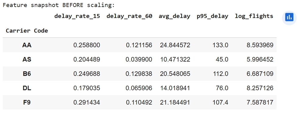
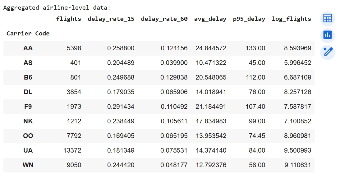
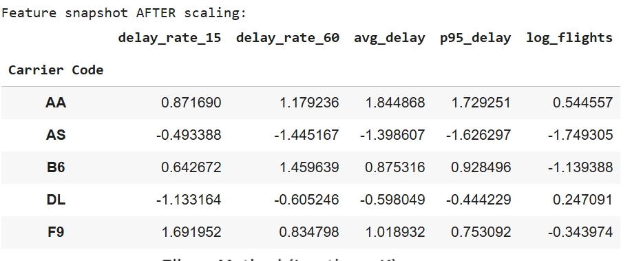
To prepare the dataset for K-Means clustering, preprocessing steps were applied to make the data compatible with the algorithm and enable fair airline comparisons. Flight-level records were first cleaned by converting delay fields to numeric values and clipping negative delays (early departures) to zero, followed by creating binary indicators for moderate (≥15 min) and severe (≥60 min) delays. Because the research question focuses on differences between airlines rather than individual flights, data was aggregated by carrier to compute total flights, delay rates, mean positive delay minutes, and the 95th percentile delay duration, while removing airlines with fewer than 50 observations. To prevent high-volume airlines from dominating cluster formation, flight count was log-transformed, and the final feature set—delay_rate_15, delay_rate_60, avg_delay, p95_delay, and log_flights—was standardized using StandardScaler so all variables contributed proportionally to the Euclidean distance calculations used by K-Means.
The performance of the K-Means model was evaluated using the Silhouette Score and the Davies-Bouldin Index. With K = 2, the model achieved a Silhouette Score of 0.500, indicating good cohesion within clusters and clear separation between them. The Davies-Bouldin Index of 0.687 further supports strong cluster quality, since lower values imply greater separation and less overlap. Together, these metrics confirm that K-Means effectively identified two meaningful airline performance groups: consistently on-time carriers vs. delay-prone carriers.
View Notebook: Models 3, 4 & 9 — Milestone 3
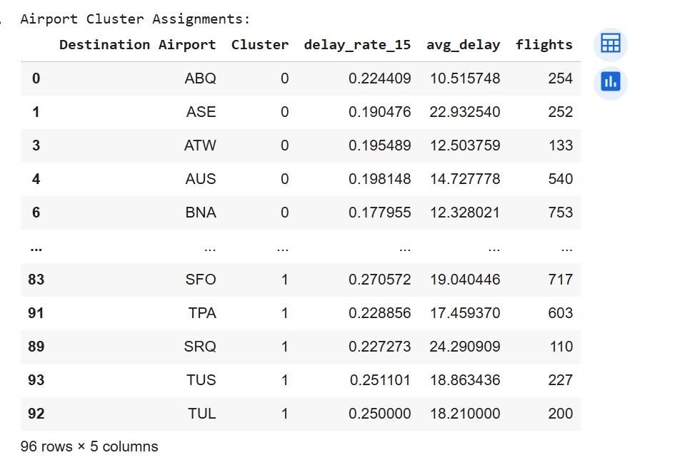
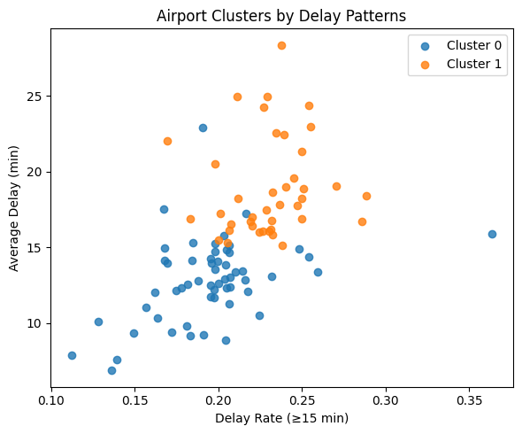
Model Choice: K-Means clustering was selected to identify groups of airports that share similar delay characteristics like frequency, duration, and underlying causes. K-Means is an appropriate unsupervised algorithm to detect groupings without predefined labels because the dataset include continuous numeric features like average delay minutes and percentage of flights delayed. This method helps highlight airports with consistently higher delay rates compared to those operating more efficiently.
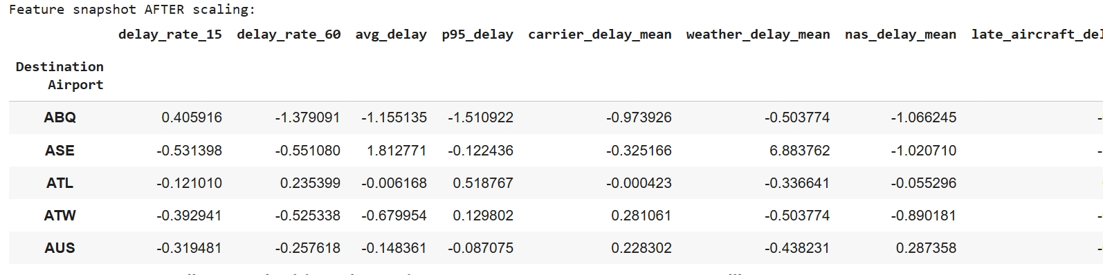
Model Assumption: K-Means requires numerical features on a comparable scale, so all inputs were standardized before clustering. This ensures Euclidean distance reflects true similarity between airlines rather than differences in variable magnitude, allowing the model to form meaningful groups.
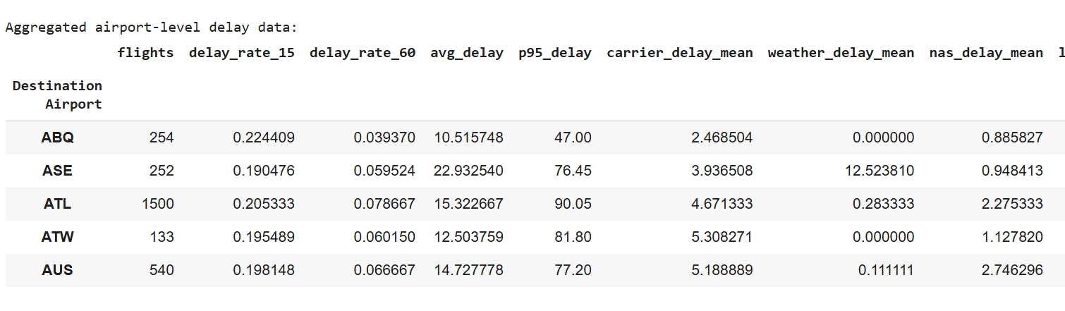
Data Preparation: To prepare the data for K-Means clustering, flight-level records were cleaned and aggregated into airport-level metrics. Delay fields were converted to numeric format and negative delays were clipped to zero. New features were engineered, including delay rates (≥15 and ≥60 minutes), mean delay duration, 95th-percentile delay, and average delay by cause. Airports with fewer than 100 flights were removed to reduce noise. Finally, all selected features were standardized so they contributed equally to Euclidean distance, and the resulting scaled feature matrix was used as input for clustering.

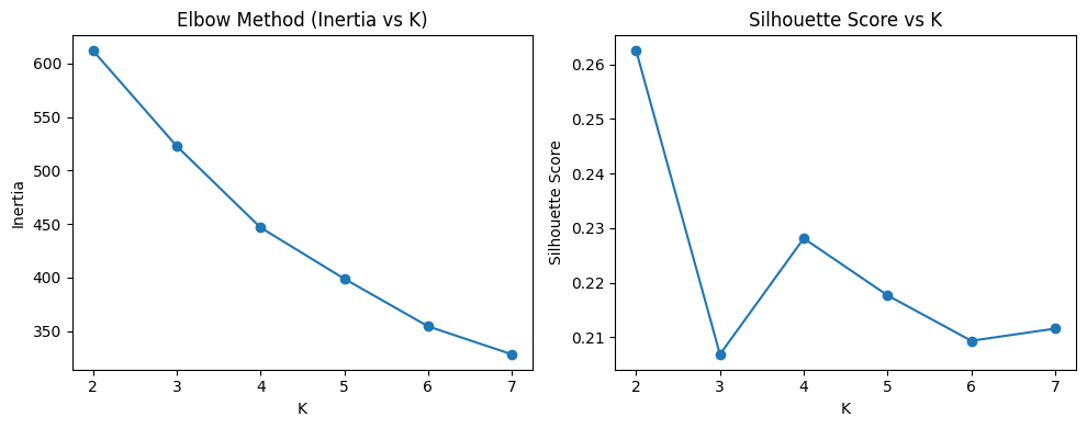
Hyperparameters Tuning: Hyperparameter tuning was conducted using both the Elbow Method and the Silhouette Score to determine the optimal number of clusters. The Elbow curve showed diminishing gains in inertia beyond K = 2, and the Silhouette curve also peaked at K = 2 with a value of 0.263. Based on these results, the final model parameters were set to n_clusters = 2, n_init = 20, and random_state = 42. The evaluation metrics (Silhouette = 0.263 and Davies–Bouldin = 1.409) indicate moderate separation between clusters, which is reasonable for real-world transportation data where delay patterns naturally overlap.
Challenges & Solutions: Several preprocessing challenges were addressed to ensure meaningful clustering. First, uneven flight volumes meant large hubs could dominate delay statistics, so a log-transformed flight count feature (log_flights) was added to balance scale differences. Second, airports with very few observations introduced noise, so locations with fewer than 100 flights were removed. Finally, extreme delay events and multiple overlapping delay causes inflated averages, so the 95th-percentile delay (p95_delay) and averaged cause-specific delay measures were used to stabilize the inputs and reduce the influence of outliers.
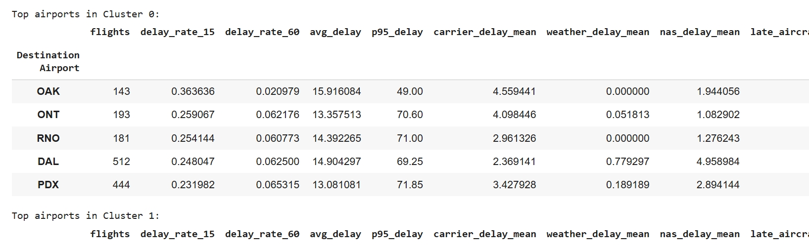
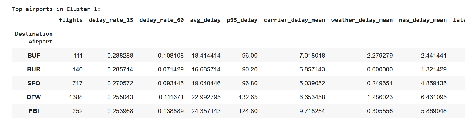
Performance & Evaluation: The K-Means clustering model performed reliably in separating airports into two delay-behavior groups. With K = 2, the model achieved a Silhouette Score of 0.263 and a Davies-Bouldin score of 1.409, indicating moderate separation between clusters. Despite natural noise in transportation systems, the model was still able to differentiate airports with consistently low delays from those with frequent and longer disruptions, demonstrating that K-Means was effective for uncovering patterns in airport delay performance.
View Notebook: Models 3, 4 & 9 — Milestone 3
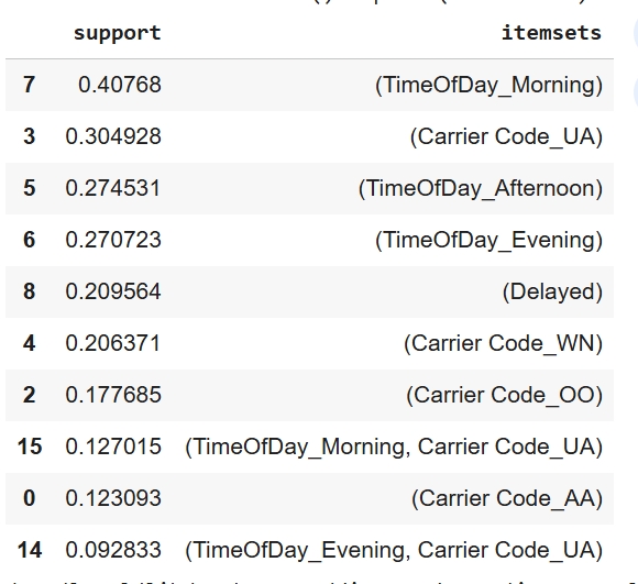
Model Choice: Apriori was applied to uncover interpretable co-occurrence patterns between categorical flight attributes and delay outcomes. The dataset of 43,853 records was well suited for a transactional format after converting departure times into time-of-day categories and one-hot encoding carrier and airport identifiers. The resulting association rules highlight clear and actionable patterns, such as certain times of day or airport characteristics that frequently co-occur with delayed departures. These insights provide an explainable layer of understanding that complements predictive modeling by identifying when and where delays are most likely to occur.
Model Assumption: The Apriori model was applied to a one-hot encoded transaction matrix containing 43,853 rows and 223 binary indicator columns. Each item is treated as an independent categorical feature, and associations are evaluated using support, confidence, and lift. The dataset produced frequent co-occurring patterns that surpassed the minimum support threshold, making it suitable for discovering meaningful relationships related to flight delays.
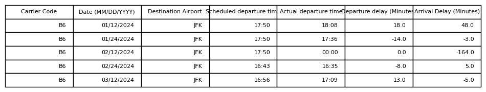
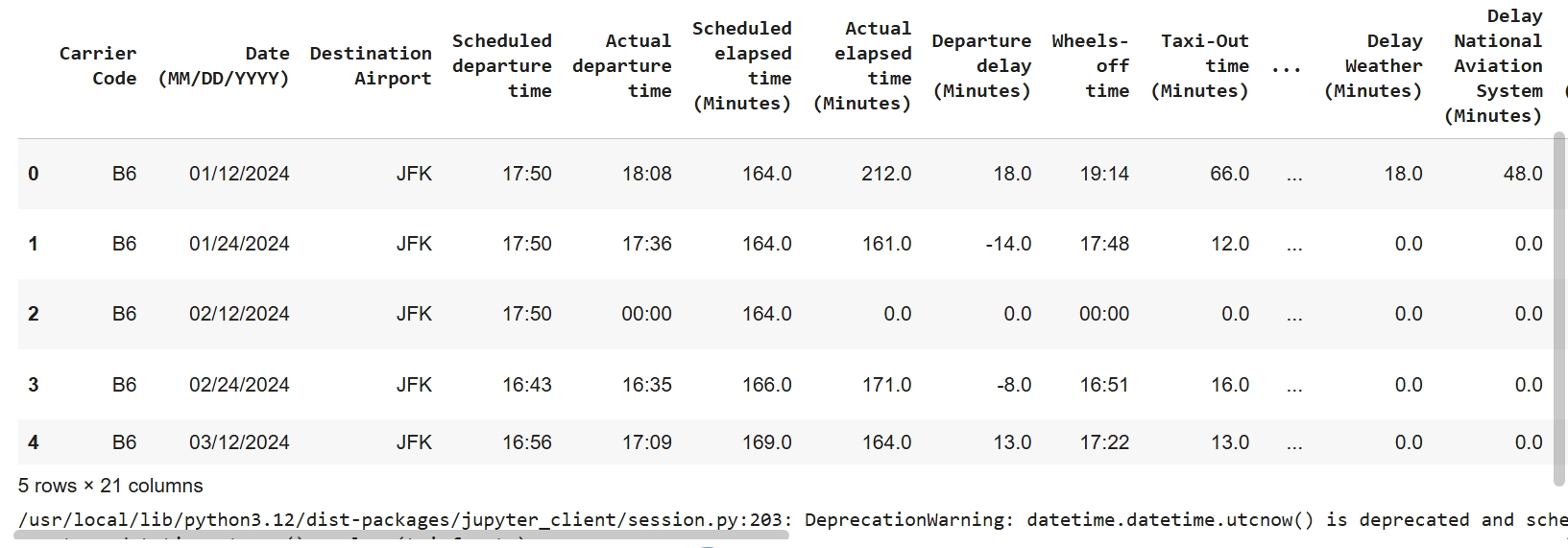
Data Preparation: To prepare the dataset for Apriori association mining, flight-level records were first cleaned and transformed into a transaction format. Departure and arrival delay fields were converted from string values to numeric, and a binary Is_Delayed flag was created to identify departures delayed by 15 minutes or more. The scheduled departure time was parsed to extract the hour of day and then bucketed into four interpretable time windows, Morning, Afternoon, Evening, and Late Night, to standardize temporal categories across flights. Categorical fields such as Carrier Code and Destination Airport were cast to string to ensure consistent encoding. A subset of relevant features (carrier, airport, time-of-day, and delay outcome) was used to generate the transaction matrix via one-hot encoding, resulting in a wide binary dataset where each column represents the presence of a category for a given flight.
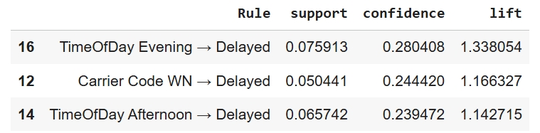
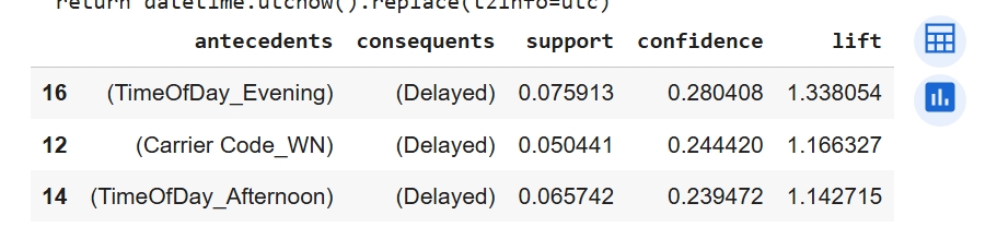
Hyperparameter Tuning:Hyperparameter tuning for Apriori used a minimum support of 0.05 to retain patterns appearing in at least 5 percent of flights, which produced 23 frequent itemsets while reducing noise. Association rules were evaluated using lift with a minimum threshold of 1.0 to ensure relationships were stronger than chance, and results were filtered to retain only rules that predicted delays. The strongest rules showed that evening departures, certain carriers, and afternoon flights were more likely to result in delays, with lift values above 1 indicating a 14 to 34 percent higher likelihood of delay compared to the baseline rate.
Challenges & Solutions: Several preprocessing issues needed to be addressed to obtain meaningful Apriori rules. The one-hot encoded transaction matrix contained 223 columns, which increased computation time and diluted support, so a minimum support of 0.05 was used to retain only meaningful patterns. Because most flights are not delayed, many trivial rules tended to predict “not delayed,” so rules were filtered to keep only those with “Delayed” as the consequent and then ranked by lift. Mixed column types initially triggered warnings and slowed execution, so the matrix was cast to boolean format to speed up mining. Finally, variability in scheduled-time strings was handled by extracting the hour and binning flights into time-of-day categories to create consistent inputs for association discovery.
Performance & Evaluation: Apriori revealed clear and interpretable patterns showing that evening flights, and to a lesser extent afternoon flights, along with certain carrier contexts, are associated with a higher likelihood of delays. These results provide insight that can support scheduling decisions, improve passenger communication, and guide staffing allocation during higher risk time periods.
View Notebook: Models 3, 4 & 9 — Milestone 3
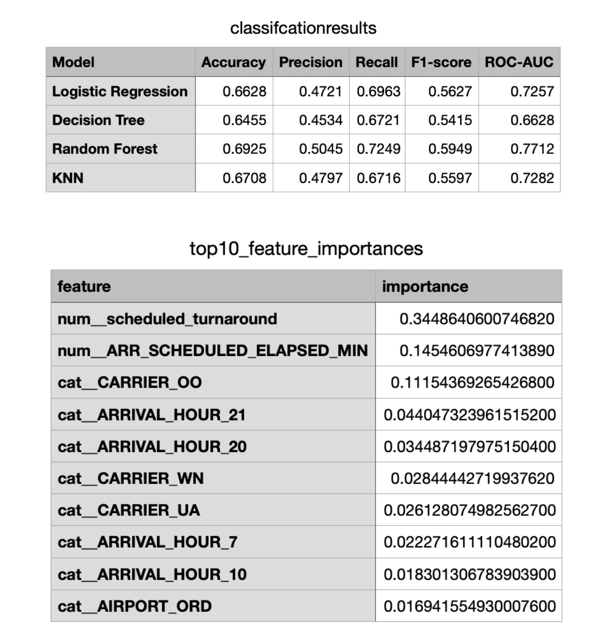
Model Choice: Based on analysis described in the data preparation section we decided to focus on predicting late aircraft delay only based on a variety of factors. Multiple models were tested such as KNN, decision tree, logistic regression and Random Forest to predict if late aircraft delay occurred. We one hot encoded the categorical attributes and scaled numerical attributes to improve performance. Random Forest gave the best performance as seen in by the metrics and was chosen as the final model for this problem.
Model Assumption: For random forest the main assumption was its ability to perform well on tasks of binary classification based on both categorical and numerical attributes which our data had.
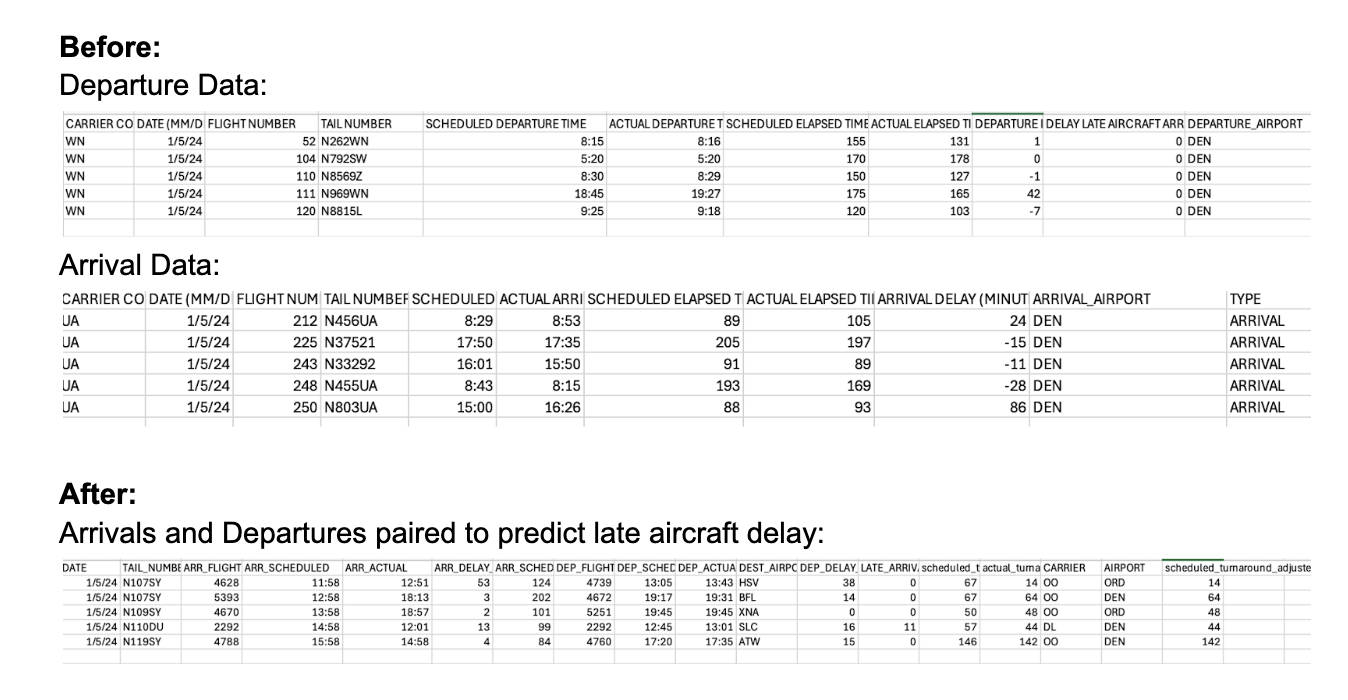
Data Preparation: Predicting delay in general is a very difficult task without real time info. After trying multiple models we concluded that delay prediction may not be possible. However, public data is available for arrivals into each airport. We already had data for departures from the previous milestone. So combining these two datasets could help classify propagation delays which are classified as Late Aircraft Delays. We merged both datasets to properly analyze information. First we find all flights under the same flight number for a given date. We then merge an arrival that occurred directly before departure for the same flight at the same airport to create a flight pair. Thus if a flight arrived late we can conclude that the departure on the same day could be affected by a Late Aircraft Delay.
Our approach for modeling was to use arriving flight info in order to determine if the departure flight had late late aircraft delay. When the arriving flight had no arrival delay the departure flight had no late aircraft delay 100 percent of the time. Thus for the model we only analyzed flight pairs where the arriving flight was delayed. This constituted about 32 percent of flights. However, while arrival delay was a strong predictor of departure delay only 30 percent of flights with arrival delay led to departure delay so our model still had work to do. Based on the data we wanted to answer two questions. Based on the occurrence of an arrival delay can we predict if a late aircraft delay will occur for the departing flight? Additionally given the exact length of the arriving flight delay can we predict how long the late aircraft delay will be?
For prediction of late aircraft delay we focused on models that help with binary classification. Most attributes were given directly from the dataset such as airline carrier, airport, time of arrival/departure, and date of arrival/departure. To simplify the model we use arrival_hour and arrival_month to give us a total of 4 categorical attributes. Additionally two numerical attributes were created. Scheduled_elapsed_time gave us an idea of the flight length and we also created a new attribute scheduled_turnaround. Scheduled_turnaround is computed as the difference between scheduled departure time and scheduled arrival time and can be a strong predictor of flight delays in real life.
Hyperparameter Tuning:Specific hyperparameters that improved performance were increasing n_estimators to 300 and min_samples_leaf which was increased to 5 to improve underfitting. Increasing past these values leads to overfitting and a decrease in model performance.
Challenges & Solutions: Note that we did not use the length of the arrival_delay as an attribute. Creating another metric called scheduled_turnaround_adjusted = scheduled_turnaround - arrival_delay could improve performance to about 82 percent. However, scheduled_turnaround_adjusted was an overpowering feature as it gave 82 percent accuracy on a single feature decision tree. Since this wasn’t insightful we decided to only use scheduled_turnaround_adjusted to predict late aircraft delay length. For classification we just used scheduled_turnaround. Despite the decrease in accuracy to 69 percent we have the additional benefit of predicting delay without having to wait for the full arrival delay. This can be seen as a large advantage in real life real time situations.
Performance & Evaluation: Our performance isn’t exceptional at 69 percent accuracy, but given the difficulty of the task and the use of arrival delay flights only it is reasonable. Based on the info above we know we can predict the majority of flights with 100 percent accuracy as they have no arrival delay. Finally, in order to evaluate the reasonability of features in random forest we looked at feature importance as seen below. It is good that multiple features such as Arrival hour, elapsed time during flight, and carrier info give important info in addition to turnaround time.
View Notebook: Late Aircraft Classification and Regression
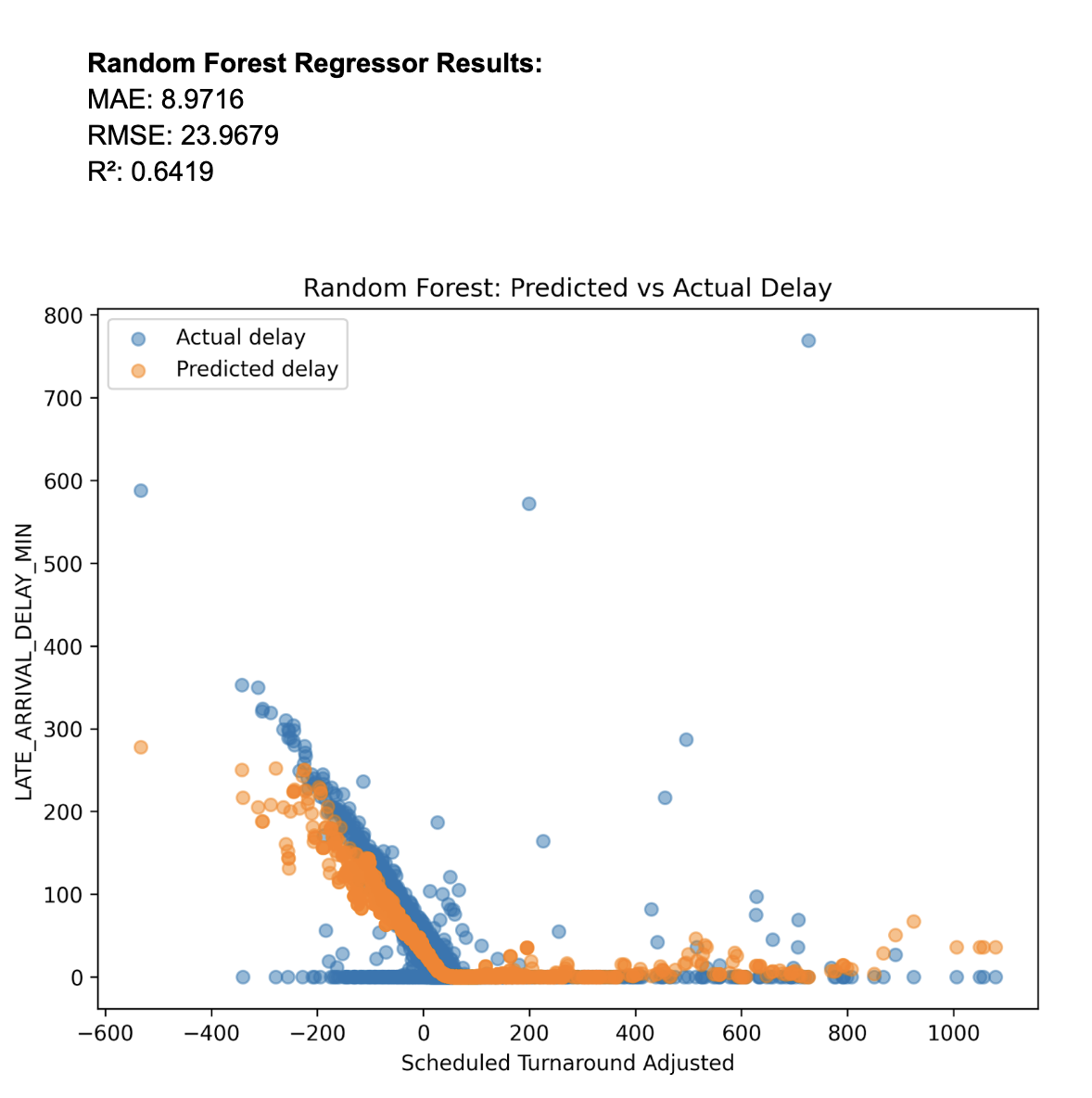
Model Choice: In order to predict the length of delay we decided to use regression since it makes the best sense to predict numerical attributes.The plots show the data as an exponential shape so we log transformed the data before using Linear Regression. Despite the transformation the results using scheduled_turnaround_adjusted to predict delay length were poor with R^2 values around 0.1. Exploring other regression models we found that Random Forest Regressor worked very well with the data as seen in results below. While we have not directly studied this model in class it is based on similar ideas as Random Forest classifier which helped motivate its usage to classification results. The basic idea of the regressor is to use a forest of decision trees where each leaf can correspond to a different section/cluster of data. Then each section/cluster can have different regression predictions based on the mean of the data in the cluster. This works well on our data as seen in the plots because there are clusters of very high delays and low delays.
Model Assumption: Random Forest regression assumes data is correlated in clusters that can be predicted by attribute branches in a decision tree. As seen from our plot it is clear we have correlation but there are clusters splitting low and high delay.
Data Preparation: Scheduled_turnaround did not perform well for regression so we used the much stronger attribute scheduled_turnaround_adjusted based on the length of the arrival delay. Dataset and preparation were identical to the late aircraft delay classification model seen earlier. The data and code link is the same as the classifier.
Hyperparameter Tuning: Hyperparameters used were identical to the classifier as this made the most sense and performed the best.
Challenges & Solutions: Other than choosing the correct regression no other challenges were encountered.
Performance & Evaluation: Results for the random forest regressor were far superior to other models even with just using scheduled_turnaround_adjusted. We can see this with the regression metrics and the plot.
Model Choice: enter body here
Model Assumption: enter body here
Data Preparation: enter body here
Hyperparameter Tuning: enter body here
Challenges & Solutions: enter body here
Performance & Evaluation: enter body here