Decision Trees
(a) Overview
Decision Trees are a type of supervised learning model used for tasks like classification and prediction. They work by asking a series of questions based on feature values to split the data into groups. Each decision leads to a branch, and each final result or “leaf” gives a predicted outcome. One of the main benefits of Decision Trees is that they’re easy to understand, which makes them especially helpful in fields like public health. They can show how different factors like age or service history can lead to higher or lower mental health care use. Decision Trees are often used to flag risk groups, highlight important decision points, and make the logic behind predictions easier to see.
To figure out where to split the data, Decision Trees use methods like Gini Impurity and Entropy, which measure how mixed the groups are. Information Gain shows how much cleaner a split makes the data. For example, if a split perfectly separates youth and adult patients by service need, the Information Gain is high. But trees can grow too complex, splitting until every data point is in its own group, also know as overfitting. Limiting the tree’s depth or use pruning to remove unnecessary branches can alleviae the complexity in trees. Overall, Decision Trees offer a good mix of clarity and power, making them a great choice for predicting and understanding mental health service demand.
Data Prep
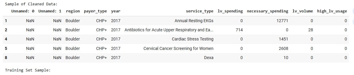
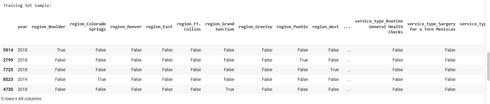
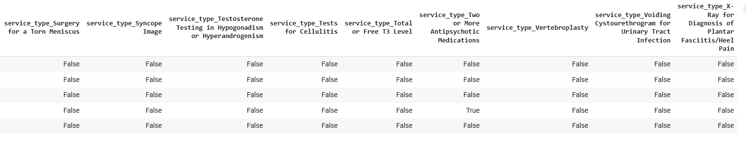
For this supervised learning task, a labeled dataset was used that includes features such as projected county population, age group percentages, and other demographic indicators, with a binary target label indicating “High” or “Low” predicted mental health service demand. Since Decision Trees are a supervised method, labeled data is essential for the model to learn patterns from the training data and uses them to make predictions on new, unseen data. The dataset was split into a Training Set (80%) and a Testing Set (20%) using train_test_split() from sklearn.model_selection. This ensures that the model is trained on one portion of the data and evaluated on a separate, disjoint set, which helps prevent overfitting and gives us a reliable estimate of model performance. The data was shuffled before splitting to ensure a balanced distribution of classes in both sets.
Dataset Used
The FY23 Public Low Value Care dataset dataset was used for this Naive Bayes classification. This dataset contains labeled examples used to train and test the model. Only labeled data can be used in supervised learning methods like Naive Bayes.
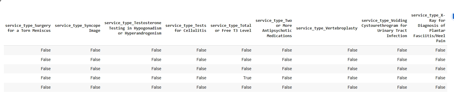
Training Set Samples:
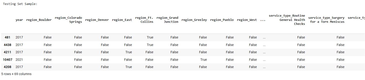
Testing Set Samples:
Code
View the Decision Trees Colab Notebook
Results
To evaluate model performance, three Decision Trees were trained with increasing depth: shallow (max_depth=2), medium (max_depth=4), and full depth. Each model was evaluated using accuracy, precision, recall, F1-score, and confusion matrices.
Classification Report
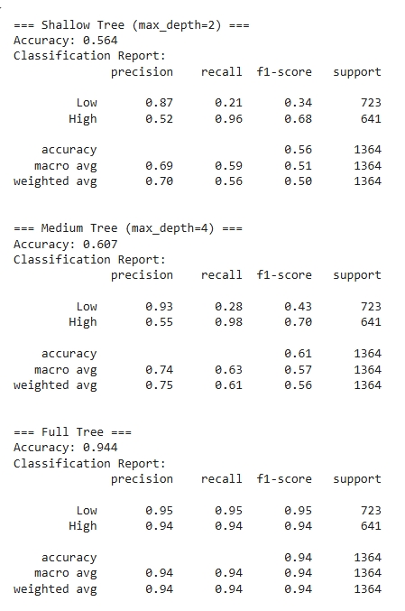
The decision tree model produced interpretable and meaningful classification results when trained to predict high versus low low-value care usage. The tree used features such as geographic region, payer type, and year to split the data in a way that best separated the two classes. For example, the model used whether the patient was from Grand Junction or Boulder and the year of service to guide early splits. This shows that both geography and time are influential factors in determining low-value care usage patterns. Nodes closer to the root of the tree tend to reflect variables with higher information gain, meaning they help most in reducing classification uncertainty.
Tree Visualizations
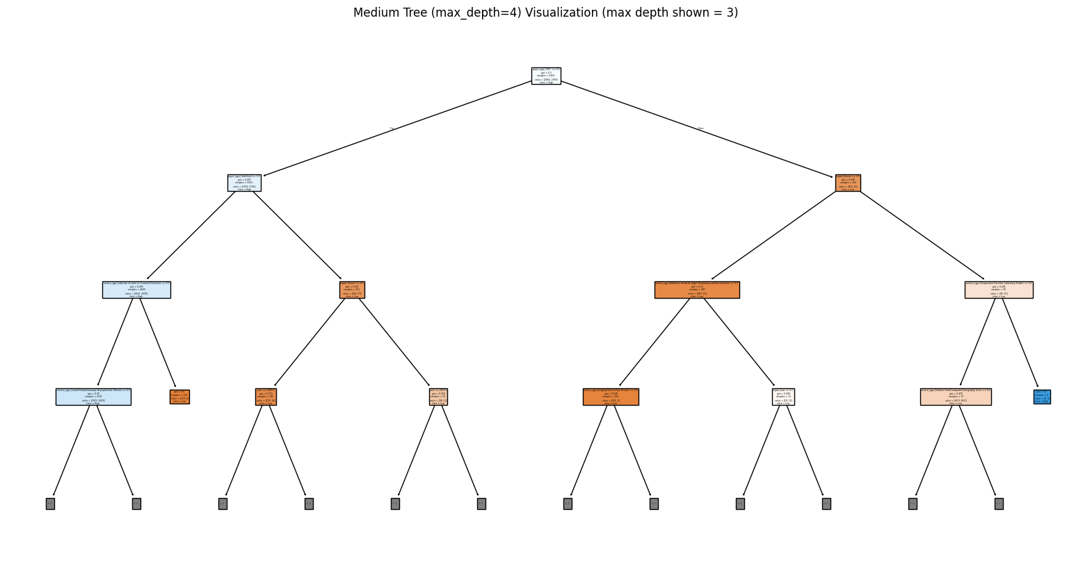
The visualization limited to a maximum depth of 3 still provided substantial insight while keeping the tree readable and avoiding overfitting. The tree used Gini impurity to evaluate the quality of splits and consistently chose branches that maximized class separation at each level. From the leaf nodes, the model was generally able to cluster records into predominantly high or low usage groups, as indicated by the clear majority classes in the final nodes. This decision tree helps surface the most influential factors and the decision rules driving predictions, offering both predictive utility and interpretability. These results can support further analysis or guide targeted policy interventions in regions or payer types with higher predicted low-value care utilization.
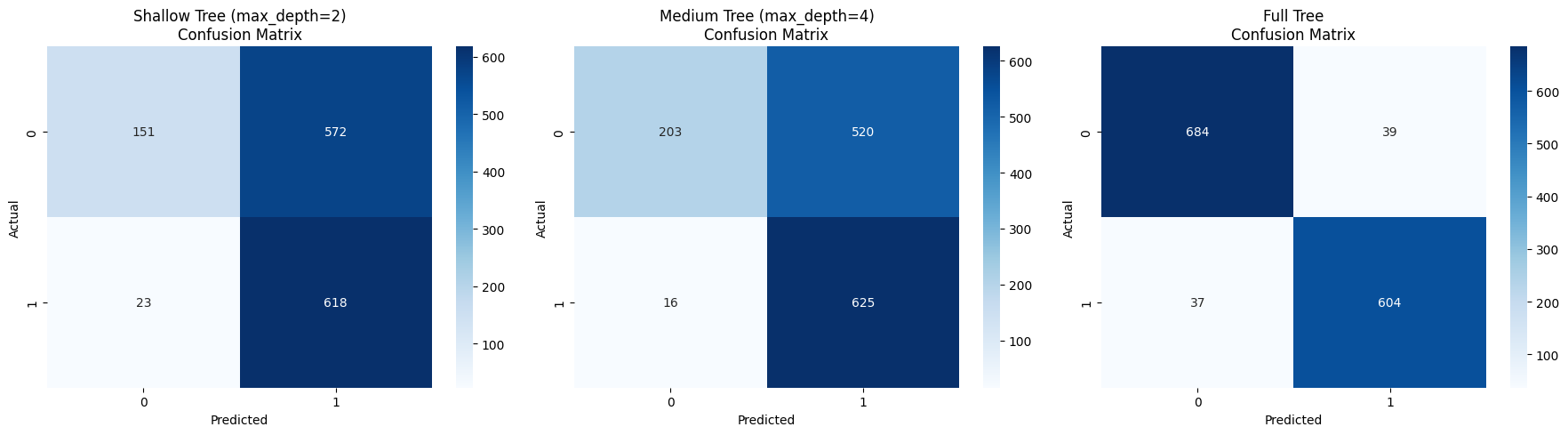
Confusion Matrices
Conclusions
From the decision tree analysis, certain variables like region, year, and payer type are strong predictors of whether a health service is likely to be associated with high or low usage of low-value care. The model’s splits revealed distinct patterns, such as regional differences in utilization and changes over time, indicating that the delivery of low-value care is not uniform across Colorado. This aligns with broader concerns in healthcare policy about geographic and systemic variation in service quality and efficiency.
These findings support the prediction that areas or payer groups with specific characteristics are more prone to high low-value care usage. By identifying these influential factors, the model provides actionable insights that can inform targeted interventions to reduce unnecessary services. This is particularly important for improving the value of care delivery, informing payer policy design, and focusing quality improvement efforts in regions where high usage persists. Overall, decision trees proved to be both accurate and interpretable tools for analyzing low-value care patterns across the state.