Neural Network
(a) Overview
A neural network is a machine learning model inspired by the human brain, made up of layers of connected nodes or neurons that process information. The input layer receives data, hidden layers transform it by applying weights, biases, and activation functions, and the output layer produces the final prediction or classification. The network learns by adjusting its weights and biases through a process called backpropagation, using optimization methods like gradient descent, so it can recognize patterns and improve its accuracy over time.
Sample CSV: sample_low_value_care_rows.csv
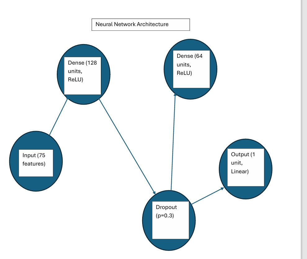
Neural Network Architecture
(b) Data Preparation
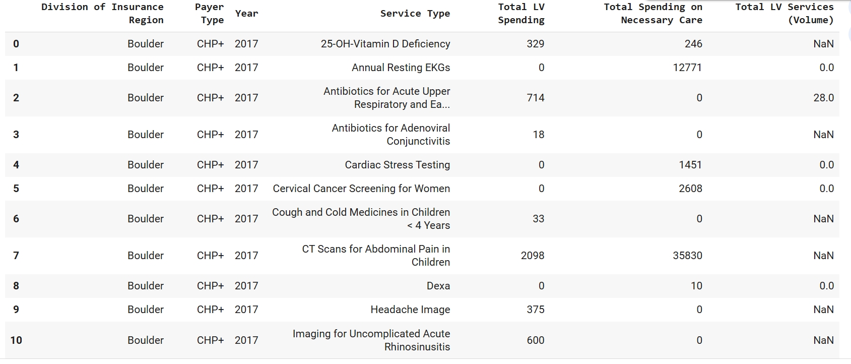
Supervised learning requires labeled data and a strict train and test separation. In this project, each row of the Low-Value Care dataset is defined by the combination of Region/ Payer/ Year/ Service, is one example. The data was prepared by cleaning currency fields, imputing missing values, one-hot encoding the categorical columns (Division of Insurance Region, Payer Type, Service Type), and scaling the numeric predictors (Year, Total Spending on Necessary Care, Total LV Services). To prevent target leakage, the target column was excluded from the feature set before preprocessing. Then a disjoint 80/20 split was created using stratification to preserve class balance. The Training Set contains 8,937 rows (Low=4,468; High=4,469) and the Testing Set contains 2,235 rows (Low=1,118; High=1,117). The training set is used solely to learn the model’s weights and the testing set is held out until final evaluation to provide an unbiased estimate of generalization. The final input matrix after encoding and scaling has 75 features.
Sample of cleaned data
Train/Test split (disjoint sets)
.png)
With the binary classifier, the label is defined as High (1) vs Low (0) Total LV Spending, using the median of Total LV Spending on the full dataset as the threshold. The neural network is therefore configured with one hidden layer (ReLU) and a single output logit, trained with BCEWithLogitsLoss and applies the sigmoid internally. This matches the requirement of one output for a binary label and makes it straightforward to report test accuracy and a confusion matrix from the held-out set.
(c) Code
Notebook: Part 5 of Final Project (Neural Network)
(d) Results
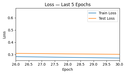
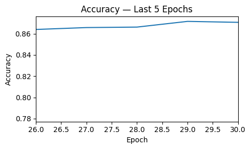
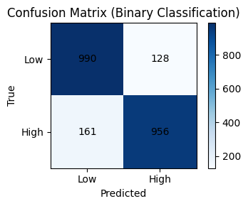
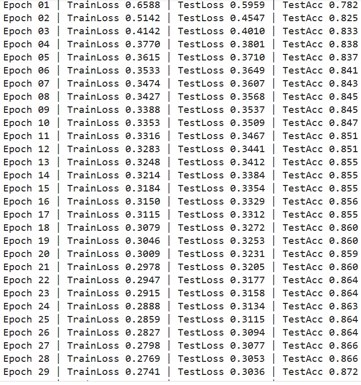
Across 30 epochs, the one-hidden-layer classifier converged smoothly. Training and test loss declined in parallel and test accuracy climbed over the final five epochs. On the held out test set, the model achieved 87.1% accuracy. The confusion matrix shows TN = 990, FP = 128, FN = 161, and TP = 956, indicating strong performance on both classes with slightly more false negatives than false positives. This pattern suggests the model is a bit more conservative on predicting “High” spending but overall generalizes well without obvious overfitting.
Loss — last 5 epochs
Accuracy — last 5 epochs
Confusion matrix (binary classification)
For interpreting the results for Low-Value Care, the network is reliably distinguishing High vs Low total LV spending using only region, payer, year, service type, and a small set of numeric predictors. To push performance further, richer features like lagged utilization by service, regional socioeconomic indicators could be engineered or tuning the decision threshold away from 0.5 to balance FN/FP to aid in policy improvement. Overall, this is a strong baseline that meets classification requirements and produces clear, actionable test-set performance.
Epoch log screenshot
(e) Conclusions
The analysis shows that a neural network can capture meaningful patterns in Low-Value Care spending when fed detailed, cleaned, and structured tabular data. Using 75 input features spanning geography, payer type, time, and service characteristics, the regression baseline achieved R² = 0.436, indicating substantial explanatory power for Total LV Spending. More importantly for decision making, a binary classification task (High vs. Low spending by median threshold), the one-hidden-layer model reached 87.1% test accuracy and produced a well-balanced confusion matrix, showing it can reliably flag higher-spend cases. While these predictions are not yet precise enough for line-item budgeting, they provide actionable signals about which combinations of region, payer, year, and service type are most associated with elevated LVC spending which is useful for prioritizing audits and interventions. This work confirms that neural networks are a viable tool for forecasting and triaging LVC patterns in Colorado, and it sets a strong foundation for future improvements by incorporating socioeconomic indicators, historical utilization, and provider-level features to further boost accuracy and policy relevance.
Test predictions (CSV): lvc_test_predictions.csv